cp.async on Ampere: Hide HBM Latency on A100
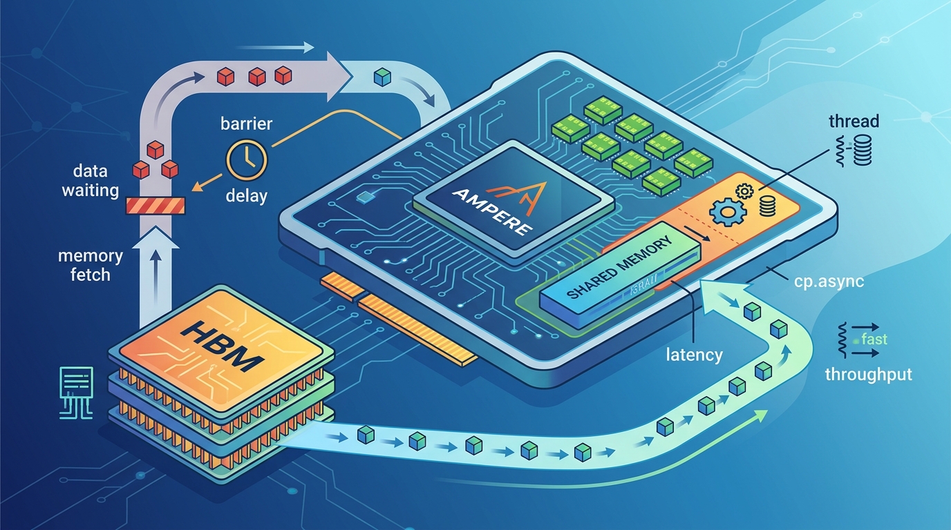
Ampere’s cp.async moves data without stalling warps, cutting HBM waits from 450–600 cycles into overlapped compute on A100.
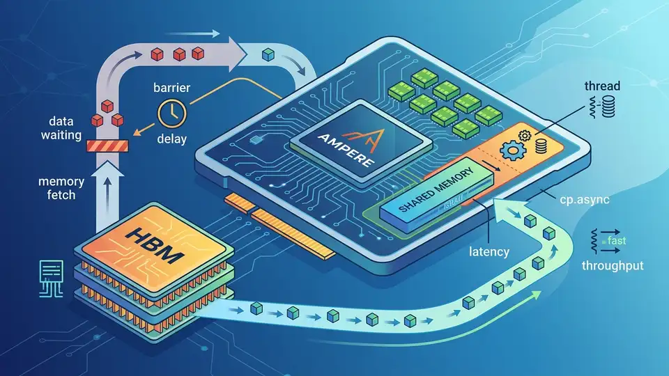
On an NVIDIA A100, an HBM2e load can cost roughly 450 to 600 cycles, which is long enough to leave an entire warp scheduler idle if you do nothing else. Ampere’s cp.async changes that by moving data into shared memory without tying up registers or setting the long scoreboard.
This is why the instruction matters: it lets the programmer describe what data should move, while the hardware handles when the transfer completes. Part VII of Mastering CUDA and High-Performance Computing is really about that shift in mental model, from blocking loads to overlapped pipelines.
The memory hierarchy on A100 is the real story
Get the latest AI news in your inbox
Weekly picks of model releases, tools, and deep dives — no spam, unsubscribe anytime.
No spam. Unsubscribe at any time.
The article opens by grounding the discussion in the A100 SXM4 memory stack, and the numbers are worth keeping in your head. Registers are fast, but they are capped at 255 per thread. Shared memory and L1 share a 192 KB pool. L2 is 40 MB. HBM2e tops out at 2 TB/s on paper, while real kernels usually land somewhere lower depending on access pattern quality.
That hierarchy is not just trivia. It explains why a kernel that looks fine in source code can fall apart in practice. If the compiler spills registers, those values go to local memory and pay the same global-memory penalty as any other DRAM access. If shared memory access patterns hit the same bank, the warp serializes. If the working set misses L2, the kernel ends up paying hundreds of cycles per access.
- Register file per SM: 256 KB total, or 64 KB per SMSP
- Shared memory bank count: 32 banks, 4 bytes wide each
- L2 cache size on A100: 40 MB split into two 20 MB slices
- HBM2e peak bandwidth: 2 TB/s theoretical, about 1.6 to 1.9 TB/s in strong cases
- HBM2e latency: roughly 450 to 600 cycles with caches bypassed
Those numbers matter because they define the gap cp.async is trying to close. Ampere is not removing latency. It is making latency easier to hide.
Why cp.async changes the execution model
Traditional global loads write into registers first. That means the warp cannot use those destination registers until the data returns, and the scheduler marks them pending. With cp.async, the copy goes straight from global memory into shared memory through a dedicated asynchronous copy engine. No destination registers are occupied. No long scoreboard bits are set for the destination data path.
That detail sounds small until you trace what it means for scheduling. The warp issues the copy, hands the transaction off, and immediately becomes eligible for more instructions. The load and the compute no longer have to happen one after the other. They can overlap.
Here is the practical effect: instead of waiting 500 cycles for memory before doing useful work, a kernel can spend those cycles computing on the previous tile while the next tile is already in flight. That is the whole point of the instruction.
“Latency hiding is the name of the game.” — Mark Harris, NVIDIA, in his CUDA programming guidance and talks on overlapping data movement with computation
Harris has repeated that idea for years, and cp.async is one of the cleanest examples of it in hardware. The programmer still needs to structure the work carefully, but the architecture gives a much better tool than the old load-store-register path.
Commit, wait, and the double-buffer pattern
The article’s explanation of commit and wait groups is the part many CUDA programmers should read twice. cp.async.commit_group does bookkeeping only. It marks a batch of copy instructions as a group. cp.async.wait_group N blocks until at most N groups remain pending. With N=1, one group can still be in flight while the kernel computes on the previous one.
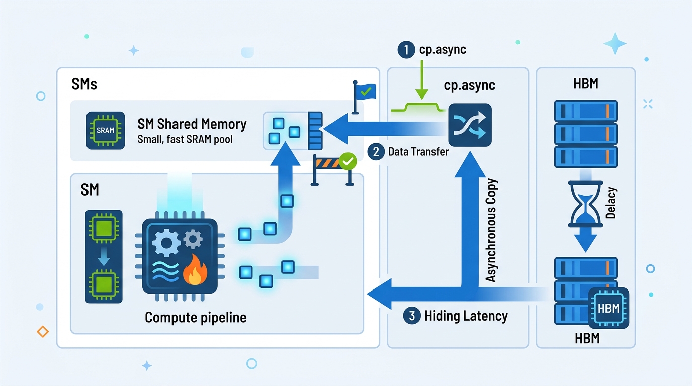
That is what turns asynchronous copy into a pipeline. You keep one buffer being filled while another buffer is being consumed. The kernel does not try to make memory faster. It keeps the machine busy while memory is slow.
- Conventional load path: load into registers, wait on long scoreboard, then store to shared memory
cp.asyncpath: copy directly into shared memory, no destination register stallcp.async.commit_group: groups prior async copies for bookkeepingcp.async.wait_group 1: allows one in-flight group while compute continues
The article also points out that this is not free. Shared memory usage rises as you add stages to the pipeline, and that can reduce occupancy. On Ampere, the best stage count depends on the kernel. A GEMM kernel with enough arithmetic intensity may benefit from multiple stages, while a lighter kernel may lose more to reduced occupancy than it gains from deeper pipelining.
That tradeoff is why libraries such as CUTLASS expose the pipeline depth as a tuning parameter. The right answer is usually measured, not guessed.
What the profiler shows before and after
The most useful part of the piece is the profiler framing. It gives you a way to tell whether your kernel is memory-stalled or actually doing work. Before pipelining, a conventional load-heavy kernel often shows long scoreboard stalls dominating the timeline. After a good cp.async rewrite, those stalls shrink and the FMA pipe stays busy for a much larger share of cycles.
That is a cleaner way to think about optimization than just chasing raw bandwidth. A kernel can look fast on paper and still waste half its issue slots waiting on memory. Once the transfer is asynchronous, the metric that matters is overlap, not just throughput.
- Before pipelining:
smsp__warp_issue_stalled_long_scoreboardoften dominates at 40% to 70% - After pipelining: long scoreboard stalls can drop below 5%
- Well-tuned kernels:
smsp__pipe_fma_cycles_activecan rise into the 70% to 90% range - A100 L2 bandwidth: about 4 TB/s aggregate, around 15x HBM bandwidth
If you want to see this in practice, look at kernels built with NVIDIA CUDA Samples and then compare them with a tiled implementation that uses asynchronous copy. The difference is usually obvious in the profiler even before you inspect the assembly.
For a broader performance view, the NVIDIA Nsight Compute documentation is the best companion piece. It shows how to read the stall reasons, issue activity, and memory throughput counters that tell you whether your pipeline is actually doing its job.
What this means for Hopper and beyond
The summary line from the source article gets to the heart of it: Ampere still leaves a programmer-visible gap between expression and execution, and Hopper reduces that gap further with TMA, or Tensor Memory Accelerator. That matters because every step in this direction makes memory movement feel less like a blocking operation and more like a scheduled transfer handled by the chip itself.
My read is simple: if you are still writing CUDA kernels that assume load, wait, compute, repeat, you are leaving a lot of performance on the table. The real question is whether your data movement can be expressed as a pipeline. If it can, cp.async is worth the extra bookkeeping. If it cannot, you may need to change the data layout first.
For developers already working on Ampere, the next move is practical: profile one hot kernel, measure long scoreboard stalls, then try a double-buffered cp.async version before touching anything else. If the stall profile drops and occupancy stays healthy, you have your answer. If not, the bottleneck is probably somewhere else, and the profiler will tell you where to look next.
That is the useful lesson here. The hardware is giving you a better way to overlap memory and compute, but it still rewards precise thinking. The teams that get the most out of Ampere and Hopper will be the ones that treat data movement as a pipeline problem, not a load instruction problem.
// Related Articles
- [RSCH]
How VLMs Learned Complex Scene Descriptions
- [RSCH]
Visual Pretraining Beats Text-Only in Language Models
- [RSCH]
PHINN-EEG brings topology to dream-state EEG
- [RSCH]
Google’s Android Bench update exposes Gemini’s gap
- [RSCH]
Benchmarks should not pick your LLM in 2026
- [RSCH]
Rust Breaks Into TIOBE’s Top 10